Take your SQL from Good to Great: Part 3

This is part 3 of a 4-part series on some of my most valued SQL ‘hacks’. Check out the others in the series:

• Part 1: Common Table Expressions
• Part 2: All about those dates
• Part 3: The other JOINs
• Part 4: Window Functions

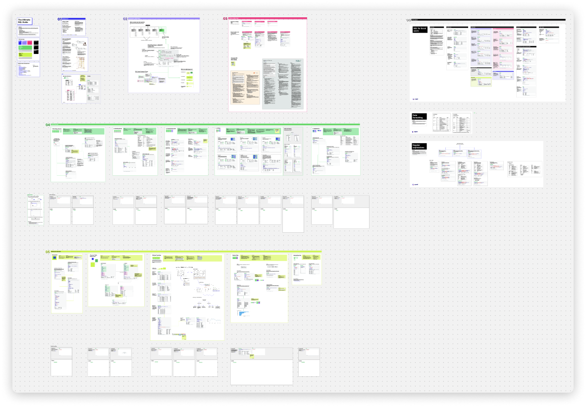
Update: Many of the concepts covered here (and more) have been assembled into The Ultimate SQL Guide, which you can see here.

The Humble JOIN

JOINs aren’t anyone’s favorite part of SQL. They aren’t as flashy as window functions or as transformational as CTEs. And yet, they’re arguably our most powerful tool to access and transform relational data.

So before getting into my favorite ways to use JOINs, I thought I’d remind myself why we should be paying more attention to the long-overlooked JOIN.

1. Optimization Power

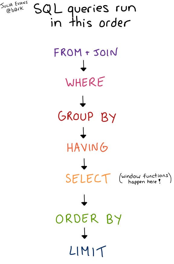
SQL queries don’t run in the order in which they’re written (or read). In fact, the SELECT statement is one of the last steps that’s completed when a query is run.

The first part of the query that’s run is the FROM/JOIN clause, meaning if we want to improve query performance (and who doesn’t), we should look first at our old friend the JOIN.

2. Creative Problem Solving

The other, and less technical reason I appreciate JOINs is that they allow us to think about our data analysis far more creatively. They act like studs on our lego blocks, allowing us to build something far greater than our database of individual tables could do on their own.

This kind of power and flexibility is one of the main reasons we still use relational databases today, despite them being nearly 50 years old.

The Default JOIN

Despite the plethora of JOIN types available to us, most people default to the LEFT JOIN. And there are some very valid reasons for that. We (in the Western world) read from left to right, it’s easier for us to conceptualize adding columns from the second table we mention, and it tends to be less computationally expensive.

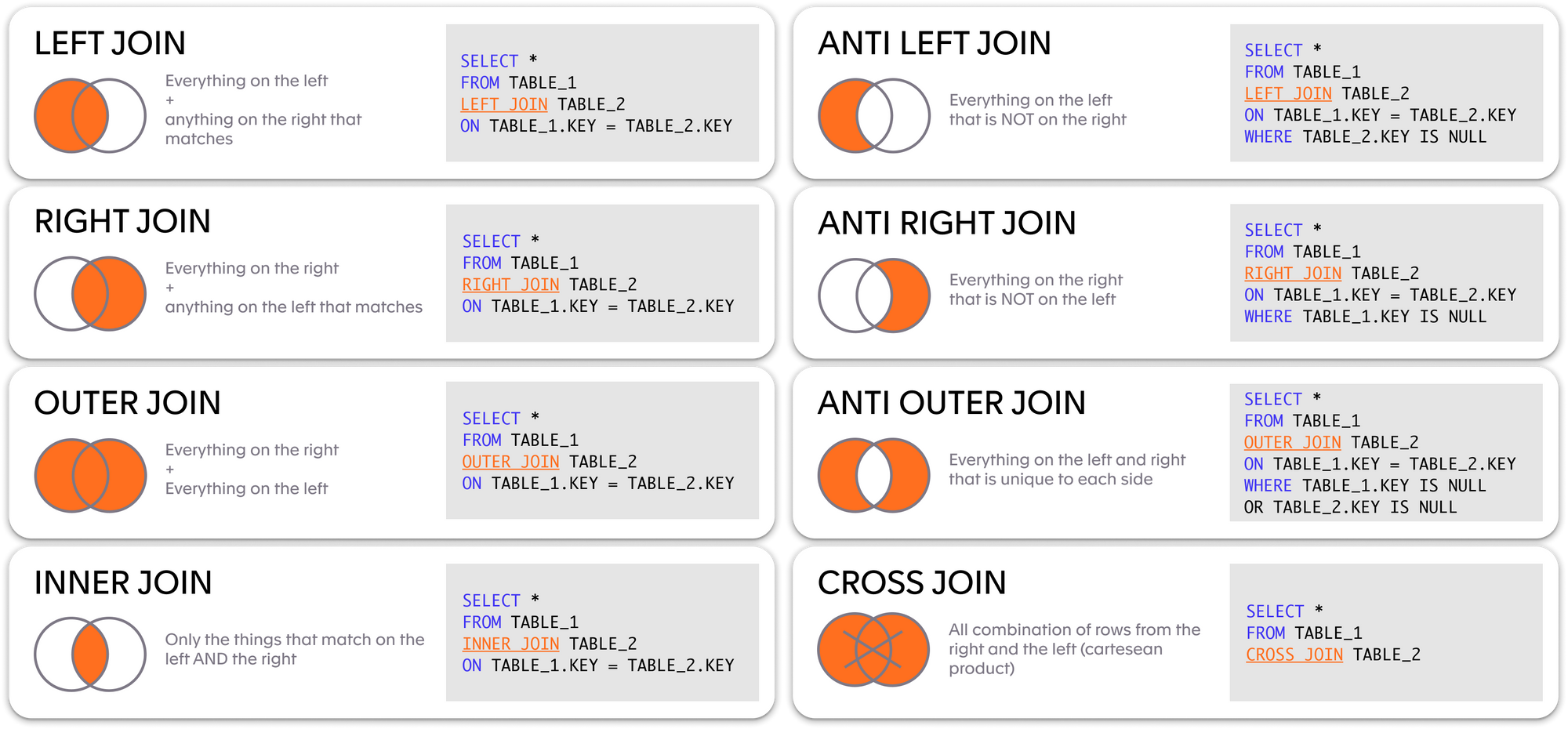
But there are scenarios where chaining together a string of LEFT JOINS might be more effort, and more computationally expensive than you can afford. For those scenarios, we can look to some of the more overlooked JOIN types:

The JOIN functionality you aren’t using enough

1. INNER JOIN instead of filtering out NULLS

Often I see people do something like:

SELECT ...
FROM X
LEFT JOIN Y
ON X.KEY = Y.KEY
WHERE Y.KEY IS NOT NULL

This effectively finds only the things that tables X and Y have in common (a.k.a. an INNER JOIN.)

SELECT ...
FROM X
INNER JOIN Y
ON X.KEY = Y.KEY

Why I like it: It’s just right. But more specifically, it’s more efficient since you don’t need as many WHERE statements, it’s faster and easier to type, and easier for others to understand. This isn’t a hack per se as much as a reminder of the fact that INNER JOIN exists and can often take care of a lot of filtering for you.

Example:

If I wanted to find the daily Spotify streams for the top 10 most streamed songs, I could:

• Find the top 10 most streamed songs
• Join that back to our daily stream data using an INNER JOIN:

In this example, the above version of the query (with top_tracks INNER JOIN daily_streams) takes 0.9 seconds to process 27 MB in BigQuery.

The LEFT JOIN option (daily_streams LEFT JOIN top_tracks…WHERE…) takes 1.9 seconds to process 27 MB.

While these are both quick, you can see how this can scale to larger data.

2. Range JOINs

When we think of joins we tend to think only of equalities, e.g. key == key. But often we need a more refined logic to merge two tables together.

For this we can do a range join, or really a join on an inequality. For example:

SELECT ...
FROM X
LEFT JOIN Y 
ON X.KEY >=Y.RANGE_START AND X.KEY <= Y.RANGE_END

Why I like it: These are really great when you need to join two tables based on some time logic. Think about trying to find the instances when your users did X after they bought their first product, or finding all the actions that occurred within their free trial window. All of these would be painful, if not outright impossible without range joins.

Example:

Let’s continue with our Spotify data and say we want to find the daily streaming data for our top tracks but only for the 30 days after the track was released.

You can see in this example, we simply extended our first example by adding a few more conditions to our INNER JOIN to make sure we were only selecting data within 30 days of the track's release date.

Warning: Not every SQL dialect supports JOINing ON inequalities. This is pretty alarming to me, but still a good idea to check before you start trying it out and getting a vague error. Then switch to a new SQL dialect.

3. Lateral JOINs

I’m relatively late to the Lateral Join party, but I have to say I like what I’ve seen so far. It took me a while to work out exactly what they were, but essentially there are 2 keys to understanding a lateral join:

1. They allow us to access columns after the FROM statement.
2. They operate like A FOR EACH operator since they are evaluated for each row of the query.

Why I like it: The ability to do FOR EACH operation in SQL is very handy, especially when you need to generate new rows for each row in your base table.

Additionally, lateral joins allow you to build off of yourself within the same query, simplifying the query logic. There are two examples of this kind of logic consolidation here and here.

Example:

To keep with Spotify, let’s say we wanted to find the top 5 tracks for each of the top 10 Spotify artists.

To do that we can:

1. Find the top 10 Artists
2. FOR EACH Artist, find their top 5 tracks using a LATERAL JOIN:

You could do this with a window function too, which just so happens to be the next topic in the series!

Warning: Not every SQL dialect has a notion of LATERAL JOINs. BigQuery uses implicit Lateral Joins via UNNEST, for example. Check your tool’s docs before trying it out for yourself!

All of the examples used were built in Count, the SQL notebook built for analysts. You can interact with the examples here:

Lateral JOINs in PostgreSQL

The Joys of Joining

Until next time, when we cover Window Functions!